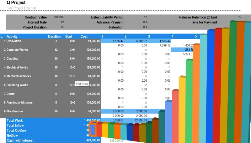
Construction Project Cash Flow Prediction

Overview of the Process

To predict a construction project's cash flow accurately, follow these steps:

1. Divide the project into activities : Break the work into specific, manageable parts.
2. Specify start and end dates : Define when each activity begins and ends.
3. Estimate costs : Assign a cost to each activity.
4. Distribute activity costs over time : Spread costs across the duration of the activity.
5. Sum costs vertically per unit time : Add up all activity costs at each time point to get the project’s cash flow.

The Problem with Linear Distribution

When cash flow is distributed evenly (linearly), it does not reflect reality because activities rarely progress in straight lines. Actual work typically follows skewed distribution curves , influenced by multiple variables:

1. Subcontracting percentage
2. Advance payments and their recovery
3. Retention payments and their release
4. Defect liability periods
5. Billing in excess of work performed
6. Payment delays

In addition, work activities rarely progress uniformly. Instead, they align with S-curves (cumulative cash flow curves), which better simulate the nature of work progression.

Using Mathematical Models for Accurate Predictions

1. Polynomial Model

The polynomial model (Formula 1) is cubic in nature:

$$f(x)=-\frac{2h}{w^3}\cdot x^3+\frac{3h}{w^2}\cdot x^2$$

Analysis :

• Purpose : Models work progression smoothly over time.
• Components :
  • $h$ : Total value of work or cash flow.
  • $w$ : Total project duration.
  • $x$ : Time variable (from 0 to $w$ ).
• Behavior :
  • At $x = 0$ , $f(x) = 0$ (start of the project).
  • At $x = w$ , $f(x) = h$ (completion of the project).
• Shape : The curve starts slowly, rises rapidly in the middle, and flattens as the project ends. This symmetric behavior reflects typical construction progress.

Limitations :

• Does not naturally account for early or late work progress without skewing.

2. Exponential Model (Skewed Curve)

The exponential model (Formula 2) introduces a skew factor $c$ :

$$f(x) = \frac{1}{(c+1) + e^{-\left(\frac{x}{0.1 \cdot w} + c^2 - 5\right)}} h (c+1)$$

Analysis :

• Purpose : Captures skewed progress for early or late activity completion.
• Components :
  • $c$ Skew factor. Positive $c$ delays progress; negative $c$ accelerates it.
  • $h$ : Total work or cash flow.
  • $w$ Project duration.
• Behavior :
  • The exponential term $e^{-k}$ reduces over time, causing $f(x)$ to asymptotically approach $h$ .
  • The skew factor $c$ shifts the curve left (early progress) or right (delayed progress).

Comparing Linear vs. Mathematical Models

1. Linear Distribution

• Description : Work progresses at an even rate across the activity duration.
• Pros : Simple to calculate and understand.
• Cons : Inaccurate because work in construction projects typically accelerates and decelerates over time.

2. Mathematical Models

• Polynomial Models : Provide smooth and realistic curves but are symmetric (cannot account for skewed progress).
• Exponential Models : More flexible as they include skew factors to simulate early or late progress.

Advantages of Skewing Curves

1. Reflect Reality : Skewed curves account for activity-specific behavior, such as slow starts (e.g., mobilization) or accelerated ends.
2. Improved Accuracy : Better aligns cash flow with actual work progress.
3. Resource Planning : Helps finance coordinators anticipate cash demands more precisely.
4. Mitigates Risk : Reduces surprises in cash shortages or delays caused by inaccurate forecasts.

Analyzing formula 1:

$$f(x) = -\frac{2h}{w^3} \cdot x^3 + \frac{3h}{w^2} \cdot x^2$$

Analysis :

1. Purpose :

   • This polynomial predicts the cashflow or work performed over time.
   • It is cubic and quadratic in nature, providing a smooth curve to model the gradual rise and eventual leveling off of work or cashflow.

2. Components :

   • $h$ : The total value of the cashflow or work to be completed.
   • $w$ : The project duration or scaling factor.
   • $x$ : Time variable (ranging from 0 to $w$ ).

3. Behavior :

   • At $x = 0$ (start of the project):
     $f(0) = 0$ → The work starts at zero.
   • At $x = w$ (end of the project):
     Substituting $x = w$ into the formula: $$f(w) = -\frac{2h}{w^3} \cdot w^3 + \frac{3h}{w^2} \cdot w^2 = -2h + 3h = h$$
   • $$$$
     Thus, at the project's end, the total work performed or cashflow is $h$ .

4. Shape :

   • The cubic term $-\frac{2h}{w^3} \cdot x^3$ dominates initially and drives the curve upward.
   • The quadratic term $\frac{3h}{w^2} \cdot x^2$ ensures the curve decelerates as it approaches $h$ .

   This combination gives the curve a concave-downward shape , where:

   • The curve starts at zero,
   • Rises steadily,
   • Slows down and approaches $h$ asymptotically at $x = w$ .

5. Comparison to Other Models :

   • Unlike exponential models, this curve is symmetric and deterministic, with no skewing.
   • It cannot model early or late progression naturally without an additional skewing parameter (like $c$ we introduce later).

Analyzing formula 2:

$$f(x)=\frac{1}{(c+1)+e^{-(\frac{x}{0.1\cdot w}+c^2-5)}}h(c+1)$$

based on the structure of the formula and its resemblance to sigmoid or logistic curves often used in project management, the parameter $c$ likely acts as the skew or shift factor of the curve. Here's why:

1. The exponential term $e^{-\left( \frac{x}{0.1 \cdot w} + c^2 - 5 \right)}$ :

   • The $\frac{x}{0.1 \cdot w}$ part controls the rate of growth or decay of the curve over time, meaning $w$ adjusts the time scaling.
   • The $c^2 - 5$ term introduces a shift in the curve. This directly influences where the curve "starts" or "centers," making $c$ responsible for skewing the curve left or right along the $x$ -axis.

2. $h(c+1)$ term:

   • $h$ is the total value of the cashflow, scaling the entire curve up to match the total work performed or cashflow value.
   • The $(c+1)$ factor adjusts the curve's scaling based on $c$ , which further indicates that $c$ has a role in distorting or skewing the progression.

3. Behavior of the curve :

   • The denominator, $(c+1) + e^{-\left( ... \right)}$ , implies that as time ( $x$ ) progresses, the exponential term reduces (as $e^{-k} \to 0$ for large $k$ ). This drives the function $f(x)$ asymptotically toward $h(c+1)$ , representing the total value of the cashflow.

4. Intuitive meaning :

   • $c$ shifts how quickly or slowly the total work (or cashflow) accumulates over time. Positive or negative values of $c$ will skew the curve to the right or left, making it a control for early or late completion trends.

To obtain cashflow use quollnet cash flow application: Cashflowpot.com

1. cashflowpot article
2. How to create a project cash flow for contractor by quollnet

This excel file is generated by cashflowpot.com. it takes only few minutes to create something similar.

• Download free construction project cashflow in excel format